


tl;dr: solve inverse problems with latent diffusion models by mimicking degradations in the latent space


Consistent improvement of image priors over the years has led to the development of better inverse problem solvers. Diffusion models are the newcomers to this arena, posing the strongest known prior to date. Recently, such models operating in a latent space have become increasingly predominant due to their efficiency. In recent works, these models have been applied to solve inverse problems. Working in the latent space typically requires multiple applications of an Autoencoder during the restoration process, which leads to both computational and restoration quality challenges. In this work, we propose a new approach for handling inverse problems with latent diffusion models, where a learned degradation function operates within the latent space, emulating a known image space degradation. Usage of the learned operator reduces the dependency on the Autoencoder to only the initial and final steps of the restoration process, facilitating faster sampling and superior restoration quality. We demonstrate the effectiveness of our method on a variety of image restoration tasks and datasets, achieving significant improvements over prior art.
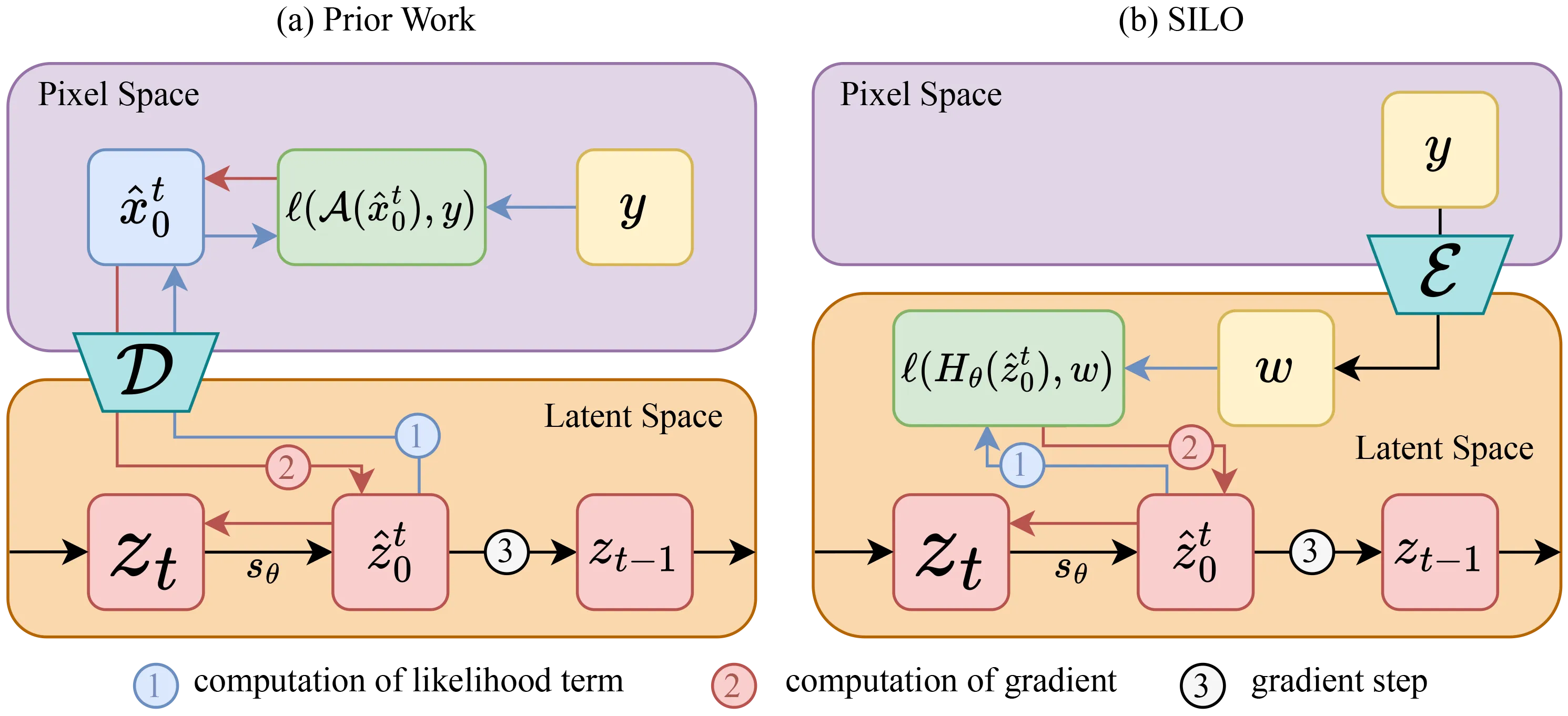
Output:
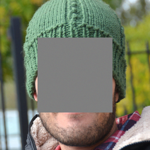
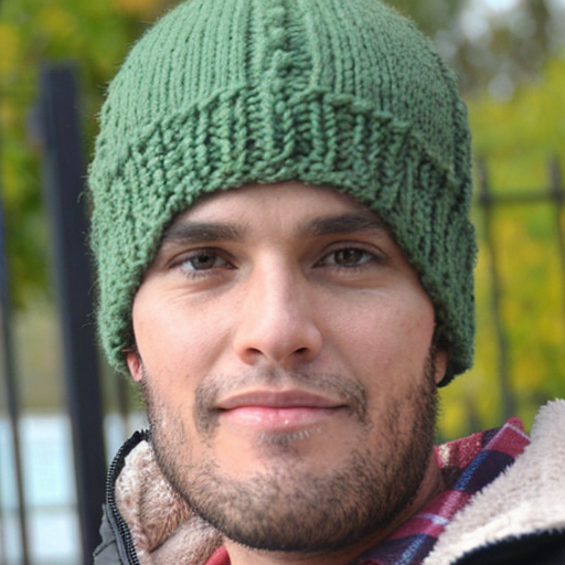
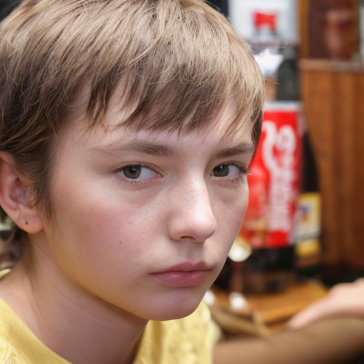
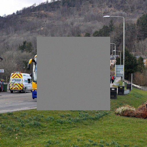
Below are some results of our method. More can be found in the paper.
| x | y | Ours (RV) | Ours (SD) | ReSample | PSLD | GML | LDPS |
|---|---|---|---|---|---|---|---|
 | |||||||
 | |||||||
 | |||||||
 | |||||||
 | |||||||
 | |||||||
 | |||||||
    @article{raphaeli2025silosolvinginverseproblems,
      title={SILO: Solving Inverse Problems with Latent Operators},
      author={Ron Raphaeli and Sean Man and Michael Elad},
      year={2025},
      journal={arXiv preprint arXiv:2501.11746},
      url={https://arxiv.org/abs/2501.11746},
}